Classification

Probability plot

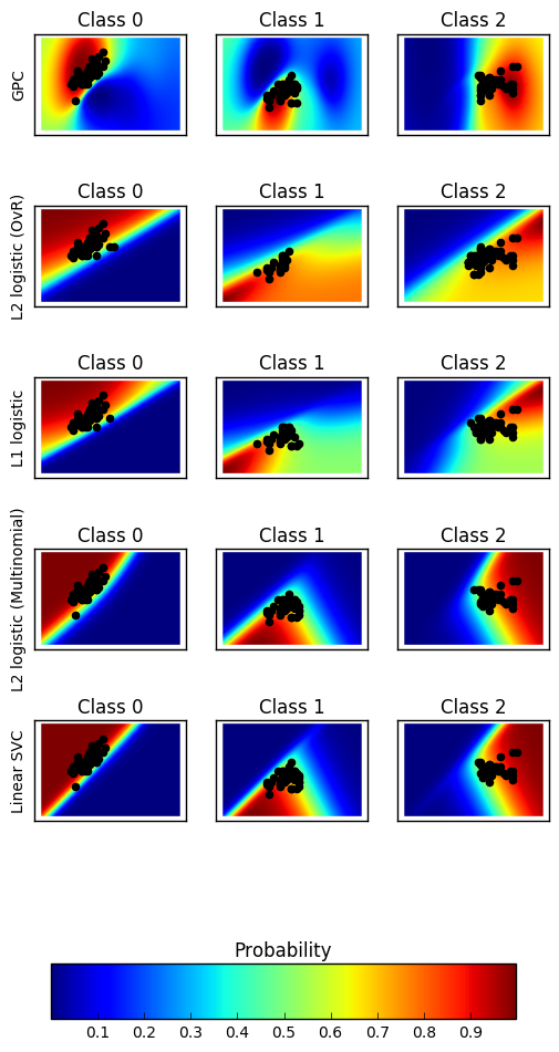
1. Plot classification probability (source)

Plot the classification probability for different classifiers. We use a 3 class dataset, and we classify it with

a Support Vector classifier (sklearn.svm.SVC),
L1 and L2 penalized logistic regression with either a One-Vs-Rest or multinomial setting (sklearn.linear_model.LogisticRegression), and
Gaussian process classification (sklearn.gaussian_process.kernels.RBF)

The logistic regression is not a multiclass classifier out of the box. As a result it can identify only the first class.

import matplotlib.pyplot as plt
import numpy as np
#========Models===================
from sklearn.linear_model import LogisticRegression
from sklearn.svm import SVC
from sklearn.gaussian_process import GaussianProcessClassifier
from sklearn.gaussian_process.kernels import RBF
#======= data set ===============================
from sklearn import datasets

Data

iris = datasets.load_iris()
X = iris.data[:, 0:2]  # we only take the first two features for visualization
y = iris.target
n_features = X.shape[1]

C = 1.0
kernel = 1.0 * RBF([1.0, 1.0])  # for GPC

# Create different classifiers. The logistic regression cannot do
# multiclass out of the box.

classifiers = {'L1 logistic': LogisticRegression(C=C, penalty='l1'),
               'L2 logistic (OvR)': LogisticRegression(C=C, penalty='l2'),
               'Linear SVC': SVC(kernel='linear', C=C, probability=True,
                                 random_state=0),
               'L2 logistic (Multinomial)': LogisticRegression(
                C=C, solver='lbfgs', multi_class='multinomial'),
               'GPC': GaussianProcessClassifier(kernel)
               }

n_classifiers = len(classifiers)

plt.figure(figsize=(3 * 2, n_classifiers * 2))
plt.subplots_adjust(bottom=.2, top=.95)

xx = np.linspace(3, 9, 100)
yy = np.linspace(1, 5, 100).T
xx, yy = np.meshgrid(xx, yy)
Xfull = np.c_[xx.ravel(), yy.ravel()]

for index, (name, classifier) in enumerate(classifiers.items()):
    classifier.fit(X, y)

    y_pred = classifier.predict(X)
    classif_rate = np.mean(y_pred.ravel() == y.ravel()) * 100
    print("classif_rate for %s : %f " % (name, classif_rate))

    # View probabilities=
    probas = classifier.predict_proba(Xfull)
    n_classes = np.unique(y_pred).size
    for k in range(n_classes):
        plt.subplot(n_classifiers, n_classes, index * n_classes + k + 1)
        plt.title("Class %d" % k)
        if k == 0:
            plt.ylabel(name)
        imshow_handle = plt.imshow(probas[:, k].reshape((100, 100)),
                                   extent=(3, 9, 1, 5), origin='lower')
        plt.xticks(())
        plt.yticks(())
        idx = (y_pred == k)
        if idx.any():
            plt.scatter(X[idx, 0], X[idx, 1], marker='o', c='k')

ax = plt.axes([0.15, 0.04, 0.7, 0.05])
plt.title("Probability")
plt.colorbar(imshow_handle, cax=ax, orientation='horizontal')

plt.show()

classif_rate for GPC : 82.666667 
classif_rate for L2 logistic (OvR) : 76.666667 
classif_rate for L1 logistic : 79.333333 
classif_rate for L2 logistic (Multinomial) : 82.000000 
classif_rate for Linear SVC : 82.000000

png

Decision boundaries

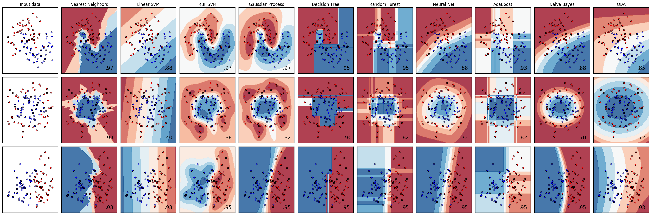
2. Classifier comparison (source)

A comparison of a several classifiers in scikit-learn on synthetic datasets. The point of this example is to illustrate the nature of decision boundaries of different classifiers. This should be taken with a grain of salt, as the intuition conveyed by these examples does not necessarily carry over to real datasets. Particularly in high-dimensional spaces, data can more easily be separated linearly and the simplicity of classifiers such as naive Bayes and linear SVMs might lead to better generalization than is achieved by other classifiers.

The plots show training points in solid colors and testing points semi-transparent. The lower right shows the classification accuracy on the test set.

Models:

sklearn.tree.DecisionTreeClassifier
sklearn.naive_bayes.GaussianNB
sklearn.neighbors.KNeighborsClassifier
sklearn.gaussian_process.GaussianProcessClassifier
sklearn.gaussian_process.kernels.RBF
sklearn.svm.SVC
sklearn.ensemble.RandomForestClassifier
sklearn.ensemble.AdaBoostClassifier
sklearn.discriminant_analysis.QuadraticDiscriminantAnalysis
sklearn.neural_network.MLPClassifier

import numpy as np
import matplotlib.pyplot as plt
from matplotlib.colors import ListedColormap

#============= preprocessing ===========================
from sklearn.model_selection import train_test_split
from sklearn.preprocessing import StandardScaler

#============= models====================================
from sklearn.neural_network import MLPClassifier
from sklearn.neighbors import KNeighborsClassifier
from sklearn.svm import SVC
from sklearn.gaussian_process import GaussianProcessClassifier
from sklearn.gaussian_process.kernels import RBF
from sklearn.tree import DecisionTreeClassifier
from sklearn.ensemble import RandomForestClassifier, AdaBoostClassifier
from sklearn.naive_bayes import GaussianNB
from sklearn.discriminant_analysis import QuadraticDiscriminantAnalysis
#========== data set=====================================================
from sklearn.datasets import make_moons, make_circles, make_classification

h = .02  # step size in the mesh

Data preparation

X, y = make_classification(n_features=2, n_redundant=0, n_informative=2,
                           random_state=1, n_clusters_per_class=1)
rng = np.random.RandomState(2)
X += 2 * rng.uniform(size=X.shape)
linearly_separable = (X, y)

datasets = [make_moons(noise=0.3, random_state=0),
            make_circles(noise=0.2, factor=0.5, random_state=1),
            linearly_separable
            ]

Assign Classifiers

names = ["Nearest Neighbors", "Linear SVM", "RBF SVM", "Gaussian Process",
         "Decision Tree", "Random Forest", "Neural Net", "AdaBoost",
         "Naive Bayes", "QDA"]

classifiers = [
    KNeighborsClassifier(3),
    SVC(kernel="linear", C=0.025),
    SVC(gamma=2, C=1),
    GaussianProcessClassifier(1.0 * RBF(1.0), warm_start=True),
    DecisionTreeClassifier(max_depth=5),
    RandomForestClassifier(max_depth=5, n_estimators=10, max_features=1),
    MLPClassifier(alpha=1),
    AdaBoostClassifier(),
    GaussianNB(),
    QuadraticDiscriminantAnalysis()]

Plot

figure = plt.figure(figsize=(27, 9))
i = 1
# iterate over datasets
for ds_cnt, ds in enumerate(datasets):
    # preprocess dataset, split into training and test part
    X, y = ds
    X = StandardScaler().fit_transform(X)
    X_train, X_test, y_train, y_test = \
        train_test_split(X, y, test_size=.4, random_state=42)

    x_min, x_max = X[:, 0].min() - .5, X[:, 0].max() + .5
    y_min, y_max = X[:, 1].min() - .5, X[:, 1].max() + .5
    xx, yy = np.meshgrid(np.arange(x_min, x_max, h),
                         np.arange(y_min, y_max, h))

    # just plot the dataset first
    cm = plt.cm.RdBu
    cm_bright = ListedColormap(['#FF0000', '#0000FF'])
    ax = plt.subplot(len(datasets), len(classifiers) + 1, i)
    if ds_cnt == 0:
        ax.set_title("Input data")
    # Plot the training points
    ax.scatter(X_train[:, 0], X_train[:, 1], c=y_train, cmap=cm_bright)
    # and testing points
    ax.scatter(X_test[:, 0], X_test[:, 1], c=y_test, cmap=cm_bright, alpha=0.6)
    ax.set_xlim(xx.min(), xx.max())
    ax.set_ylim(yy.min(), yy.max())
    ax.set_xticks(())
    ax.set_yticks(())
    i += 1

    # iterate over classifiers
    for name, clf in zip(names, classifiers):
        ax = plt.subplot(len(datasets), len(classifiers) + 1, i)
        clf.fit(X_train, y_train)
        score = clf.score(X_test, y_test)

        # Plot the decision boundary. For that, we will assign a color to each
        # point in the mesh [x_min, x_max]x[y_min, y_max].
        if hasattr(clf, "decision_function"):
            Z = clf.decision_function(np.c_[xx.ravel(), yy.ravel()])
        else:
            Z = clf.predict_proba(np.c_[xx.ravel(), yy.ravel()])[:, 1]

        # Put the result into a color plot
        Z = Z.reshape(xx.shape)
        ax.contourf(xx, yy, Z, cmap=cm, alpha=.8)

        # Plot also the training points
        ax.scatter(X_train[:, 0], X_train[:, 1], c=y_train, cmap=cm_bright)
        # and testing points
        ax.scatter(X_test[:, 0], X_test[:, 1], c=y_test, cmap=cm_bright,
                   alpha=0.6)

        ax.set_xlim(xx.min(), xx.max())
        ax.set_ylim(yy.min(), yy.max())
        ax.set_xticks(())
        ax.set_yticks(())
        if ds_cnt == 0:
            ax.set_title(name)
        ax.text(xx.max() - .3, yy.min() + .3, ('%.2f' % score).lstrip('0'),
                size=15, horizontalalignment='right')
        i += 1

plt.tight_layout()
plt.show()

png

Digit Classifier

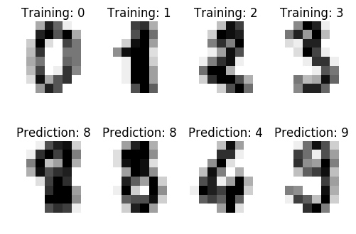
3. Recognizing hand-written digits(source)

An example showing how the scikit-learn can be used to recognize images of hand-written digits.

# Standard scientific Python imports
import matplotlib.pyplot as plt

# Import datasets, classifiers and performance metrics
from sklearn import datasets, svm, metrics

The data that we are interested in is made of 8x8 images of digits, let's have a look at the first 4 images, stored in the images attribute of the dataset. If we were working from image files, we could load them using matplotlib.pyplot.imread. Note that each image must have the same size. For these images, we know which digit they represent: it is given in the 'target' of the dataset.

The digits dataset

digits = datasets.load_digits()

To apply a classifier on this data, we need to flatten the image, to turn the data in a (samples, feature) matrix:

n_samples = len(digits.images)
data = digits.images.reshape((n_samples, -1))

Create a classifier: a support vector classifier

classifier = svm.SVC(gamma=0.001)

We learn the digits on the first half of the digits

classifier.fit(data[:n_samples / 2], digits.target[:n_samples / 2])

SVC(C=1.0, cache_size=200, class_weight=None, coef0=0.0,
  decision_function_shape=None, degree=3, gamma=0.001, kernel='rbf',
  max_iter=-1, probability=False, random_state=None, shrinking=True,
  tol=0.001, verbose=False)

Now predict the value of the digit on the second half:

expected = digits.target[n_samples / 2:]
predicted = classifier.predict(data[n_samples / 2:])

print("Classification report for classifier %s:\n%s\n"
      % (classifier, metrics.classification_report(expected, predicted)))
print("Confusion matrix:\n%s" % metrics.confusion_matrix(expected, predicted))

Classification report for classifier SVC(C=1.0, cache_size=200, class_weight=None, coef0=0.0,
  decision_function_shape=None, degree=3, gamma=0.001, kernel='rbf',
  max_iter=-1, probability=False, random_state=None, shrinking=True,
  tol=0.001, verbose=False):
             precision    recall  f1-score   support

          0       1.00      0.99      0.99        88
          1       0.99      0.97      0.98        91
          2       0.99      0.99      0.99        86
          3       0.98      0.87      0.92        91
          4       0.99      0.96      0.97        92
          5       0.95      0.97      0.96        91
          6       0.99      0.99      0.99        91
          7       0.96      0.99      0.97        89
          8       0.94      1.00      0.97        88
          9       0.93      0.98      0.95        92

avg / total       0.97      0.97      0.97       899


Confusion matrix:
[[87  0  0  0  1  0  0  0  0  0]
 [ 0 88  1  0  0  0  0  0  1  1]
 [ 0  0 85  1  0  0  0  0  0  0]
 [ 0  0  0 79  0  3  0  4  5  0]
 [ 0  0  0  0 88  0  0  0  0  4]
 [ 0  0  0  0  0 88  1  0  0  2]
 [ 0  1  0  0  0  0 90  0  0  0]
 [ 0  0  0  0  0  1  0 88  0  0]
 [ 0  0  0  0  0  0  0  0 88  0]
 [ 0  0  0  1  0  1  0  0  0 90]]

images_and_labels = list(zip(digits.images, digits.target))
for index, (image, label) in enumerate(images_and_labels[:4]):
    plt.subplot(2, 4, index + 1)
    plt.axis('off')
    plt.imshow(image, cmap=plt.cm.gray_r, interpolation='nearest')
    plt.title('Training: %i' % label)

images_and_predictions = list(zip(digits.images[n_samples / 2:], predicted))
for index, (image, prediction) in enumerate(images_and_predictions[:4]):
    plt.subplot(2, 4, index + 5)
    plt.axis('off')
    plt.imshow(image, cmap=plt.cm.gray_r, interpolation='nearest')
    plt.title('Prediction: %i' % prediction)

plt.show()

png

Discriminant Analysis

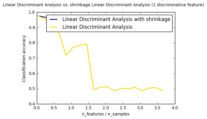
4. Normal and Shrinkage Linear Discriminant Analysis for classification(source)

from __future__ import division

import numpy as np
import matplotlib.pyplot as plt

from sklearn.datasets import make_blobs
from sklearn.discriminant_analysis import LinearDiscriminantAnalysis

n_train = 20  # samples for training
n_test = 200  # samples for testing
n_averages = 50  # how often to repeat classification
n_features_max = 75  # maximum number of features
step = 4  # step size for the calculation

def generate_data(n_samples, n_features):
    """Generate random blob-ish data with noisy features.
    This returns an array of input data with shape `(n_samples, n_features)`
    and an array of `n_samples` target labels.
    Only one feature contains discriminative information, the other features
    contain only noise.
    """
    X, y = make_blobs(n_samples=n_samples, n_features=1, centers=[[-2], [2]])

    # add non-discriminative features
    if n_features > 1:
        X = np.hstack([X, np.random.randn(n_samples, n_features - 1)])
    return X, y

acc_clf1, acc_clf2 = [], []
n_features_range = range(1, n_features_max + 1, step)
for n_features in n_features_range:
    score_clf1, score_clf2 = 0, 0
    for _ in range(n_averages):
        X, y = generate_data(n_train, n_features)

        clf1 = LinearDiscriminantAnalysis(solver='lsqr', shrinkage='auto').fit(X, y)
        clf2 = LinearDiscriminantAnalysis(solver='lsqr', shrinkage=None).fit(X, y)

        X, y = generate_data(n_test, n_features)
        score_clf1 += clf1.score(X, y)
        score_clf2 += clf2.score(X, y)

    acc_clf1.append(score_clf1 / n_averages)
    acc_clf2.append(score_clf2 / n_averages)

features_samples_ratio = np.array(n_features_range) / n_train

plt.plot(features_samples_ratio, acc_clf1, linewidth=2,
         label="Linear Discriminant Analysis with shrinkage", color='navy')
plt.plot(features_samples_ratio, acc_clf2, linewidth=2,
         label="Linear Discriminant Analysis", color='gold')

plt.xlabel('n_features / n_samples')
plt.ylabel('Classification accuracy')

plt.legend(loc=1, prop={'size': 12})
plt.suptitle('Linear Discriminant Analysis vs. \
shrinkage Linear Discriminant Analysis (1 discriminative feature)')
plt.show()

png

Discriminant Analysis

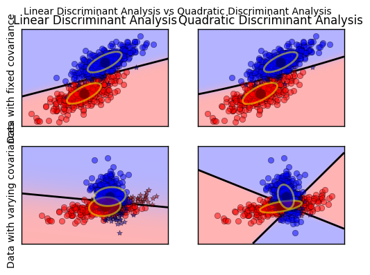
5. Linear and Quadratic Discriminant Analysis with covariance ellipsoid (source)

This example plots the covariance ellipsoids of each class and decision boundary learned by LDA and QDA. The ellipsoids display the double standard deviation for each class. With LDA, the standard deviation is the same for all the classes, while each class has its own standard deviation with QDA.

from scipy import linalg
import numpy as np
import matplotlib.pyplot as plt
import matplotlib as mpl
from matplotlib import colors

from sklearn.discriminant_analysis import LinearDiscriminantAnalysis
from sklearn.discriminant_analysis import QuadraticDiscriminantAnalysis

colormap

cmap = colors.LinearSegmentedColormap(
    'red_blue_classes',
    {'red': [(0, 1, 1), (1, 0.7, 0.7)],
     'green': [(0, 0.7, 0.7), (1, 0.7, 0.7)],
     'blue': [(0, 0.7, 0.7), (1, 1, 1)]})
plt.cm.register_cmap(cmap=cmap)

generate datasets

def dataset_fixed_cov():
    '''Generate 2 Gaussians samples with the same covariance matrix'''
    n, dim = 300, 2
    np.random.seed(0)
    C = np.array([[0., -0.23], [0.83, .23]])
    X = np.r_[np.dot(np.random.randn(n, dim), C),
              np.dot(np.random.randn(n, dim), C) + np.array([1, 1])]
    y = np.hstack((np.zeros(n), np.ones(n)))
    return X, y


def dataset_cov():
    '''Generate 2 Gaussians samples with different covariance matrices'''
    n, dim = 300, 2
    np.random.seed(0)
    C = np.array([[0., -1.], [2.5, .7]]) * 2.
    X = np.r_[np.dot(np.random.randn(n, dim), C),
              np.dot(np.random.randn(n, dim), C.T) + np.array([1, 4])]
    y = np.hstack((np.zeros(n), np.ones(n)))
    return X, y

plot functions

def plot_data(lda, X, y, y_pred, fig_index):
    splot = plt.subplot(2, 2, fig_index)
    if fig_index == 1:
        plt.title('Linear Discriminant Analysis')
        plt.ylabel('Data with fixed covariance')
    elif fig_index == 2:
        plt.title('Quadratic Discriminant Analysis')
    elif fig_index == 3:
        plt.ylabel('Data with varying covariances')

    tp = (y == y_pred)  # True Positive
    tp0, tp1 = tp[y == 0], tp[y == 1]
    X0, X1 = X[y == 0], X[y == 1]
    X0_tp, X0_fp = X0[tp0], X0[~tp0]
    X1_tp, X1_fp = X1[tp1], X1[~tp1]

    alpha = 0.5

    # class 0: dots
    plt.plot(X0_tp[:, 0], X0_tp[:, 1], 'o', alpha=alpha,
             color='red')
    plt.plot(X0_fp[:, 0], X0_fp[:, 1], '*', alpha=alpha,
             color='#990000')  # dark red

    # class 1: dots
    plt.plot(X1_tp[:, 0], X1_tp[:, 1], 'o', alpha=alpha,
             color='blue')
    plt.plot(X1_fp[:, 0], X1_fp[:, 1], '*', alpha=alpha,
             color='#000099')  # dark blue

    # class 0 and 1 : areas
    nx, ny = 200, 100
    x_min, x_max = plt.xlim()
    y_min, y_max = plt.ylim()
    xx, yy = np.meshgrid(np.linspace(x_min, x_max, nx),
                         np.linspace(y_min, y_max, ny))
    Z = lda.predict_proba(np.c_[xx.ravel(), yy.ravel()])
    Z = Z[:, 1].reshape(xx.shape)
    plt.pcolormesh(xx, yy, Z, cmap='red_blue_classes',
                   norm=colors.Normalize(0., 1.))
    plt.contour(xx, yy, Z, [0.5], linewidths=2., colors='k')

    # means
    plt.plot(lda.means_[0][0], lda.means_[0][1],
             'o', color='black', markersize=10)
    plt.plot(lda.means_[1][0], lda.means_[1][1],
             'o', color='black', markersize=10)

    return splot

def plot_ellipse(splot, mean, cov, color):
    v, w = linalg.eigh(cov)
    u = w[0] / linalg.norm(w[0])
    angle = np.arctan(u[1] / u[0])
    angle = 180 * angle / np.pi  # convert to degrees
    # filled Gaussian at 2 standard deviation
    ell = mpl.patches.Ellipse(mean, 2 * v[0] ** 0.5, 2 * v[1] ** 0.5,
                              180 + angle, facecolor=color, edgecolor='yellow',
                              linewidth=2, zorder=2)
    ell.set_clip_box(splot.bbox)
    ell.set_alpha(0.5)
    splot.add_artist(ell)
    splot.set_xticks(())
    splot.set_yticks(())


def plot_lda_cov(lda, splot):
    plot_ellipse(splot, lda.means_[0], lda.covariance_, 'red')
    plot_ellipse(splot, lda.means_[1], lda.covariance_, 'blue')


def plot_qda_cov(qda, splot):
    plot_ellipse(splot, qda.means_[0], qda.covariances_[0], 'red')
    plot_ellipse(splot, qda.means_[1], qda.covariances_[1], 'blue')

for i, (X, y) in enumerate([dataset_fixed_cov(), dataset_cov()]):
    # Linear Discriminant Analysis
    lda = LinearDiscriminantAnalysis(solver="svd", store_covariance=True)
    y_pred = lda.fit(X, y).predict(X)
    splot = plot_data(lda, X, y, y_pred, fig_index=2 * i + 1)
    plot_lda_cov(lda, splot)
    plt.axis('tight')

    # Quadratic Discriminant Analysis
    qda = QuadraticDiscriminantAnalysis(store_covariances=True)
    y_pred = qda.fit(X, y).predict(X)
    splot = plot_data(qda, X, y, y_pred, fig_index=2 * i + 2)
    plot_qda_cov(qda, splot)
    plt.axis('tight')
plt.suptitle('Linear Discriminant Analysis vs Quadratic Discriminant Analysis')
plt.show()

png